Using shapefiles on GBIF data with R
Not all filters are born equal
It happens sometimes that users need GBIF data that fall within specific boundaries. The GBIF Portal provides a location filter where it is possible to draw a rectangle or a polygon on the map and get the occurrence records within this shape. However these tools have a limited precision and occasionally the job calls for more complex shapes than the GBIF Portal currently supports.
The shapefile
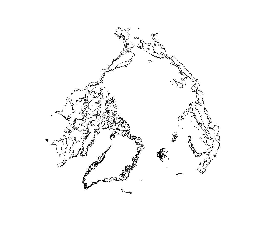
In this case I want to use a Circumpolar Arctic Map which already here is providing us with some challenges.
The map projection for this is ‘laea’ (Lambert Azimuthal Equal Area for those of you out in mercator land) and it is well suited to polar perspective.
So the task is to identify the Plant records that fall within this shape file of land areas in the Arctic region.
The arctic shape file can be downloaded here: Bioclimate subzones
The GBIF data
Since we are not going to work on GBIF data directly in the portal, we have to download a subset to work on in R. Now, the more data we grab the bigger the risk that we will blow through memory. These are the steps taken to reduce the initial GBIF data download:
- As the target is the arctic region it would be reasonable to query for all plant records above 55 degrees latitude. This returns a file of about ~35 million records. This is too large.
- Remove records within Sweden, Finland, Denmark and Great Britain.
- Filter records out that have the geospatial issues flag and now we are down to ~12 million records. Further reductions are possible with some judicious taxonomic discrimination.
The records are available from GBIF using this filtered search
The GBIF download comes with many columns but for the purpose of using the shape file we only need the coordinates and the unique record ID. More on this later. Due to the size of the download file the R function fread() is recommended for turning the GBIF records into a data table because it is much faster than read.table or read.csv.
gbif <- fread("arctic_plants.txt", sep = "\t", header = TRUE, na.strings = "\\N")
Putting it together in R
It would be sensible to insert a warning here that the R script relies on a suite of packages and that there could be some dependencies that need to be resolved before these will load. Make sure these are installed:
library(rgeos)
library(maptools)
library(proj4)
library(data.table)
library(rgdal)
library(dplyr)
library(raster)
Assuming the shape file archive is unpacked and in the work directory:
shpfile <- "Bioclimate_Subzones.shp"
The readOGR function from the rgdal package is used to pull the shape data into a spatial vector object in R.
Now comes a function that takes as arguments the shapefile (.shp), a data frame/data table, the three column names we need lat/long coordinates and the record ID, and lastly the datum for the GBIF records.
#'Filter georeferenced records by shapefile
#'
#' @param shapefile A shapefile object (.shp)
#' @param occurrence_df A data frame of georeferenced records. For large csv use fread()
#' @param lat The column name for latitude in the data frame
#' @param lon The column name for longitude in the data frame
#' @param gbifid A unique record key
#' @param map_crs The datum assigned to the occurrence data frame
#' @param mkplot Whether to draw the map plots. Can be very expensive
occurrence.from.shapefile <- function(shapefile, occurrence_df, lat, lon, gbifid, map_crs = "+proj=longlat +datum=WGS84", mkplot = FALSE){

    shape <- readOGR(shapefile)
    print(proj4string(shape))

    #subset the GBIF data into a data frame
    occ.map <- data.frame(occurrence_df[[lon]], occurrence_df[[lat]], occurrence_df[[gbifid]])
    print(str(occ.map, 1))
    #simplify column names
    names(occ.map)[1:3] <- c('long', 'lat', 'gbifid')
    print(head(occ.map, 10))
    #turning the data frame into a "spatial points data frame"
    coordinates(occ.map) <- c("long", "lat")
    #defining the datum
    proj4string(occ.map) <- CRS(map_crs)
    #reprojecting the 'gbif' data frame to the same as in the 'shape' object
    occ.map <- spTransform(occ.map, proj4string(shape))

    #Identifying records from gbif that fall within the shape polygons
    inside <- occ.map[apply(gIntersects(occ.map, shape, byid = TRUE), 2, any),]

    if(mkplot){
        raster::plot(shape)
        points(inside, col = "olivedrab3")
    }

    #Prepare data frame for joining with the occcurrence df so only records
    #that fall inside the polygons get selected
    res.gbif <- data.frame(inside@data)
    final.gbif <- gbif %>% semi_join(res.gbif, by = c(gbifid = "gbifid"))

    return(final.gbif)
}
A brief explanation of the CRS function used is in order; the occ.map spatial points data frame becomes associated with the Coordinate Reference System (the map_crs argument).
proj4string(occ.map) <- CRS(map_crs)
This allows us to reproject the GBIF data to the same projection that the shape file comes with which is, as mentioned above, the Lambert Azimuthal Equal Area projection.
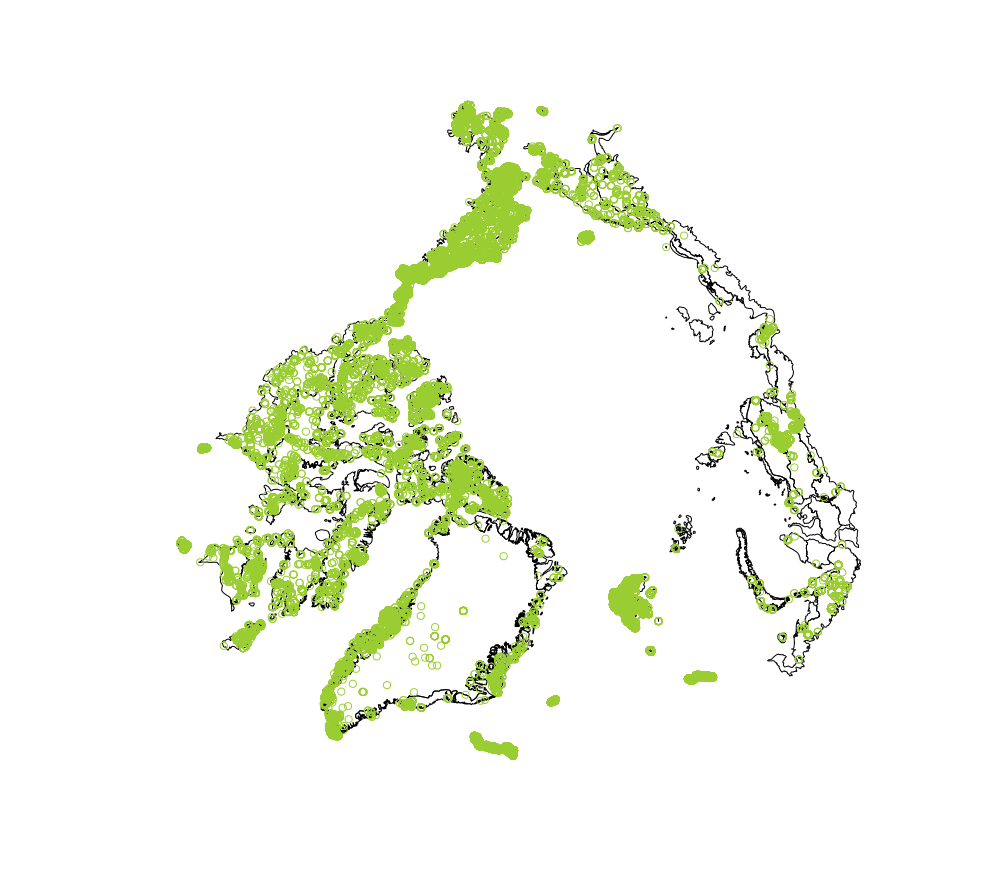
The next part of the function picks out the GBIF record IDs which are located within the polygons in the shape file. Now we are ready to join the initial GBIF records data frame with the selected GBIF IDs we have found (res.gbif) for the final data frame output. The filtered output comes to 11,108 GBIF plant records.
Of course it would be really nice to have a plot of the shape file with the occurrence records displayed. If RStudio is used the plot will render in the Plots tab when the mkplot parameter is set to TRUE.
 The complete R code can be found here.