Plot almost anything using the GBIF maps api
The GBIF maps api is an under-used but powerful web service provided by GBIF. The maps api is used by the main GBIF portal to create the maps including the big map used on gbif.org. We can make a simple call to the api by pasting the link below into a web browser.
https://api.gbif.org/v2/map/occurrence/density/0/0/0@1x.png?style=purpleYellow.point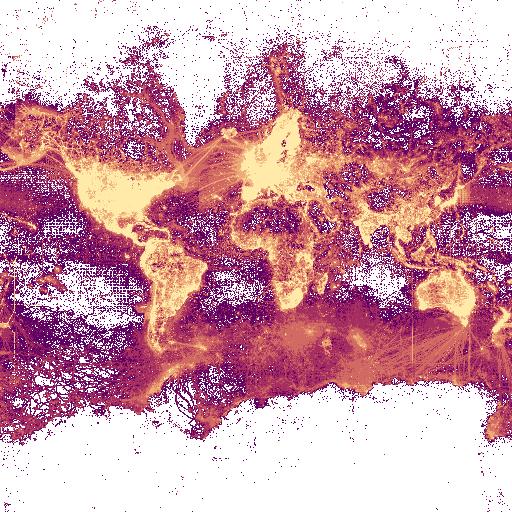
This api call is composed essentially of two elements
- a url prefix: https://api.gbif.org/v2/map/occurrence/density/0/0/0@1x.png?
- a style query: style=purpleYellow.point
This is cool but also not very interesting or useful. But the GBIF maps api is much more powerful. You don’t need to understand everything to make a cool interactive map with GBIF data. Let’s simply overlay these tiles to an existing map in R.
I will use the leaflet R package, which is a wrapper to the popular javascript library.
library(leaflet)

prefix = 'https://api.gbif.org/v2/map/occurrence/density/{z}/{x}/{y}@1x.png?'
style = 'style=purpleYellow.point'
tile = paste0(prefix,style)

leaflet() %>%
setView(lng = 20, lat = 20, zoom = 01) %>%
addTiles() %>%
addTiles(urlTemplate=tile)
A single dataset with polygons
We can also plot any dataset. Below I plot a French dataset (“Réserve Naturelle de Camargue”) without ever downloding a record.
library(leaflet)

prefix = 'https://api.gbif.org/v2/map/occurrence/density/{z}/{x}/{y}@1x.png?'
style = 'style=classic.poly&bin=hex&hexPerTile=30'
datasetKey = 'datasetKey=906b2d3f-dbd7-4c5c-acfc-c572c35c2b5a'
tile = paste0(prefix,style,'&',datasetKey)

leaflet() %>%
setView(lng = 5.4265362, lat = 43.4200248, zoom = 08) %>%
addTiles() %>% # add default map tiles
addTiles(urlTemplate=tile)
Other raster styles
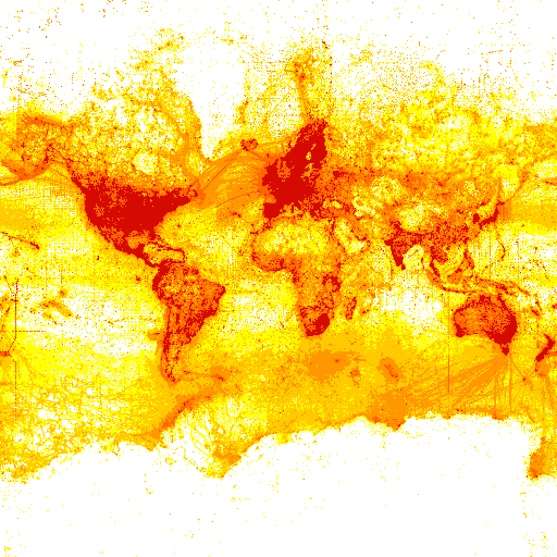
The main GBIF portal uses the raster style “gbif-violet” documented here. We can use this raster style too!
library(leaflet)

projection = '3857' # projection code.
style = 'style=gbif-violet' # style
tile = paste0('https://tile.gbif.org/',projection,'/omt/{z}/{x}/{y}@1x.png?',style)

leaflet() %>%
setView(lng = 5.4265362, lat = 43.4200248, zoom = 01) %>%
addTiles(urlTemplate=tile)
Plotting the GBIF-style eBird dataset map in leaflet using R.
We can also mimmick the plot of the largest dataset in GBIF.
library(leaflet)

# create the gbif-violet style raster layer
projection = '3857' # projection code
style = 'style=gbif-violet' # style
tileRaster = paste0('https://tile.gbif.org/',projection,'/omt/{z}/{x}/{y}@1x.png?',style)

# create our polygons layer
prefix = 'https://api.gbif.org/v2/map/occurrence/density/{z}/{x}/{y}@1x.png?'
polygons = 'style=classic.poly&bin=hex&hexPerTile=70' # ploygon styles
datasetKey = 'datasetKey=4fa7b334-ce0d-4e88-aaae-2e0c138d049e' # eBird key
tilePolygons = paste0(prefix,polygons,'&',datasetKey)

# plot the styled map
leaflet() %>%
setView(lng = 5.4265362, lat = 43.4200248, zoom = 01) %>%
addTiles(urlTemplate=tileRaster) %>%
addTiles(urlTemplate=tilePolygons)
Plotting using a taxon key
Plotting all dragonfly records.
library(leaflet)

# create style raster layer
projection = '3857' # projection code
style = 'style=osm-bright' # map style
tileRaster = paste0('https://tile.gbif.org/',projection,'/omt/{z}/{x}/{y}@1x.png?',style)

# create our polygons layer
prefix = 'https://api.gbif.org/v2/map/occurrence/density/{z}/{x}/{y}@1x.png?'
polygons = 'style=fire.point' # ploygon styles
taxonKey = 'taxonKey=789' # taxonKey of Odonata (dragonflies and damselflies)
tilePolygons = paste0(prefix,polygons,'&',taxonKey)

# plot the styled map
leaflet() %>%
setView(lng = 5.4265362, lat = 43.4200248, zoom = 01) %>%
addTiles(urlTemplate=tileRaster) %>%
addTiles(urlTemplate=tilePolygons)
Plotting any query
It is nice that we can re-create standard GBIF maps found on the portal but it would be better if we could quickly map any query ourselves and then layer in other information. This example is more complex than the examples above but also more general. By using the so-called “ad-hoc” maps api interface, we can plot complex queries without ever downloading a record.
To use the ad hoc interface with leaflet, we need to set a custom projection with leafletOptions and leafletCRS.
From the leaflet R package documentation:
The Leaflet package expects all point, line, and shape data to be specified in latitude and longitude using WGS 84 (a.k.a. EPSG:4326). By default, when displaying this data it projects everything to EPSG:3857 and expects that any map tiles are also displayed in EPSG:3857.
The GBIF ad-hoc search can only be used with EPSG:4326. Therefore, we need to define the EPSG:4326 manually. I used epsg.io to look up this projection and copied the code field PROJ.4. I then looked into the documentation and guessed that I need to use the crsClass L.CRS.EPSG4326.
library(leaflet)

# need to define new projection. Only this projection will work with custom queries.
epsg4326 <- leafletCRS(crsClass = "L.CRS.EPSG4326", code = "EPSG:4326",
            proj4def = "+proj=longlat +datum=WGS84 +no_defs",
            resolutions = 2^(10:0),
            origin =c(0,0)
            )

# create the gbif-geyser style raster layer
projection <- '4326' # must use this projection code for custom maps
style <- 'style=gbif-geyser' # I think any style will work
tileRaster <- paste0('https://tile.gbif.org/',projection,'/omt/{z}/{x}/{y}@1x.png?',style)

# create the data layer with dragonfly data # Note the "adhoc"
prefix <- 'https://api.gbif.org/v2/map/occurrence/adhoc/{z}/{x}/{y}@1x.png?'
# make query
style <- 'style=classic.poly' # style of polygons
taxonKey = 'taxonKey=789' # taxon key of Odonata
country = 'country=JP' # country code of Japan
tilePolygons = paste0(prefix,style,'&',taxonKey,'&',country)

# plot the map
leaflet(options = leafletOptions(crs = epsg4326)) %>%
setView(lng=139.068,lat=36.4910,zoom=03) %>%
addTiles(urlTemplate=tileRaster) %>%
addTiles(urlTemplate=tilePolygons) %>%
addMarkers(139.068,36.4910) # country centroid of Japan
All dragonfly occurrence records in in Japan with the country centroid of Japan marked.